Configuration¶

The json file must contain one single object named neural_network, inside which all configuration will reside:

{
    "neural_network": {
        "outfile": "log_file.txt",
        "num_epochs": 100,
        "debug": false,
        "data": {
            ...
        },
        "optimizer": {
            ...
        },
        "loss": {
            ...
        },
        "layers": {
            ...
        }
    }
}

The neural_network object contains several sub-objects (sections) which will be discussed below, in addition to a few basic parameters:

outfile: Base name for the output files produced by the run (with loss values, accuracies, etc). If not provided, no output files are created.
num_epochs: How many total epochs to run for (default: 1).
debug: Whether to write out a graph description of the neural network in .dot format (default is false).
debug_interval: How often to write out debug info (in terms of number of epochs).

Optimizer section¶

This section configures the optimizer for the neural network, which can be selected with the parameter type. RocketML supports the most important first-order algorithms available in PyTorch (module torch.optim), as well as a Hessian-based second-order optimizer. Each optimizer type has its own set of supported hyper-parameters:

SGD:
- learning_rate: Base learning rate (default: 0.01)
- momentum: Momentum factor (default: 0)
- weight_decay: Weight decay (L2 penalty) (default: 0)
- dampening: Dampening for momentum (default: 0)
- nesterov: Enables Nesterov momentum (default: false)
Adagrad:
- learning_rate: Base learning rate (default: 0.01)
- lr_decay: Learning rate decay (default: 0)
- weight_decay: Weight decay (L2 penalty) (default: 0)
Adam and AdamW:
- learning_rate: The base learning rate (default: 0.01)
- beta1 and beta2: Coefficients used for computing running averages of gradient and its square (defaults: 0.9 and 0.999)
- weight_decay: weight decay (L2 penalty) (default: 0)
- eps: Term added to the denominator to improve numerical stability (default: 1e-8)
- amsgrad: Whether to use the AMSGrad variant of this algorithm (default: false)
RMSprop:
- learning_rate: Base learning rate (default: 0.01)
- momentum: Momentum factor (default: 0)
- alpha: Smoothing constant (default: 0.99)
- eps: Term added to the denominator to improve numerical stability (default: 1e-8)
- centered: If true, compute the centered RMSProp, and normalize the gradient by its variance (default: false)
- weight_decay: Weight decay (L2 penalty) (default: 0)
LARS (see https://arxiv.org/pdf/1708.03888.pdf):

SGD-based first-order optimizer suitable for large-batch training. It accepts all parameters of the SGD optimizer, plus the LARS coefficient:
- eta: LARS’s coefficient $\eta$ , or trust-ratio multiplier (default: 1e-3)
LAMB (see https://arxiv.org/pdf/1904.00962.pdf):

Adam-based first-order optimizer suitable for large-batch training. It accepts all parameters of the Adam optimizer.
Hessian:
- max_iterations: Maximum number of iterations (default: 2000)
- max_func_eval: Maximum number of objective function evaluations (default: 4000)
- absolute_tolerance: Absolute tolerance (default: 1e-8)
- relative_tolerance: Relative tolerance (default: 1e-8)

Therefore, a typical example of invoking the Adagrad optimizer would look like this:

"optimizer": {
    "type": "Adagrad",
    "learning_rate": 0.001,
    "lr_decay": 1e-5
}

LR scheduler sub-section¶

An optional learning rate scheduler can be attached to the optimizer in order to automatically adjust the learning rate during training. This can be accomplished by adding a lr_scheduler section under the optimizer section in the configuration. For example, to engage an exponential decay scheduler to the Adam optimizer, one can do:

"optimizer": {
    "type": "Adam",
    "learning_rate": 0.01,
    "lr_scheduler": {
        "type": "Exponential",
        "gamma": 0.2,
        "verbose": true
    }
}

In this case, the learning_rate parameter will control the initial LR value, which will then be adjusted by the scheduler at the end of each epoch.

The following LR schedulers are currently supported in rmldnn:

Step LR: Decays the learning rate by $\gamma$ at every step_size epochs.

{ "type": "Step", "gamma": 0.1, "step_size": 2 }
Multi-step LR: Decays the learning rate $\gamma$ once the number of epoch reaches one of the milestones.

{ "type": "MultiStep", "gamma": 0.1, "milestones": [2,5,20,50] }
Exponential LR: Decays the learning rate by $\gamma$ at the end of every single epoch.

{ "type": "Exponential", "gamma": 0.1 }
Warmup LR: Sets the initial learning rate to start_factor * learning_rate, where start_factor < 1, then scales it up for the next num_epochs until it reaches learning_rate.

{ "type": "Warmup", "num_epochs": 5, "start_factor": 0.2 }

Layers section¶

This section allows for detailed specification of all layers in the neural network, as well as the connections between them. The syntax is supposed to follow closely the one used by Keras, which allows exporting a programmatically built neural network as a json file – see the Keras documentation. Not all functionality exposed by Keras has been integrated into RocketML, though, either due to being low priority, or because they would require support for different network architectures not currently available in rmldnn.

One can either put the network description on a separate file (e.g., model.json) and pass the file name to RocketML configuration,

"layers": "../path/model.json"

or enter it directly as an array of json objects, one for each layer:

"layers": [
    {
        "class_name": "Conv2D",
        "config": {
            "name": "layer1",
            "trainable": true,
            ...
        }
    },
    {
        "class_name": "MaxPooling2D",
        "config": {
            "name": "layer2",
            "trainable": true,
            ...
        }
    },
    ...
]

The configuration parameters available for each layer are, of course, specific to the functionality of that particular layer. Please refer to the Keras documentation for details. For example, a two-dimensional convolutional layer is represented in Keras by a Conv2D object, which accepts the following configuration parameters, among others:

filters: The number of channels of the output (i.e., number of output filters in the convolution)
kernel_size: An integer or list of 2 integers specifying the height and width of the 2D convolution window
strides: An integer or list of 2 integers specifying the strides of the convolution along the height and width
padding: An integer or list of 2 integers specifying the amount of zero-padding along the height and width. Also accepts a string with either same or valid (Tensorflow notation)
dilation_rate: An integer or list of 2 integers specifying the dilation rate to use for dilated convolution
use_bias: A boolean indicating whether the layer uses a bias vector
trainable: If set to false, the layer gets frozen, i.e., its parameters are not updated during training. This can be applied to all trainable layers (not only Conv2d), and might be useful when loading a pre-trained model.

Therefore, in order to add such a layer to the network in RocketML, the following json object could be used:

{
    "class_name": "Conv2D",
    "config": {
        "name": "conv_layer_1",
        "filters": 64,
        "kernel_size": [7, 7],
        "strides": [2, 2],
        "padding": "valid",
        "dilation_rate": [1, 1],
        "use_bias": true
        "activation": "ReLU",
        "trainable": true
    },
    "inbound_nodes": [
        [
            [
                "input_1",
                0,
                0,
                {}
            ]
        ]
    ]
}

The parameter inbound_nodes is used to indicate which layers feed into conv_layer_1. If not specified, RocketML assumes that the output of the previous layer becomes the input of the next layer. This parameter can be a list of layers, which must all feed into a so-called merge layer, which then combines the incoming data tensors into a single tensor (via either concatenation, addition, or subtraction).

Loss section¶

This section specifies which loss function to use for the neural network. The loss function computes some kind of metric that estimates the error (loss) between the network result for a given input and its corresponding target.

The choice of loss function must be consistent with the network design, in particular, with the last layer in the network and its activation. For example, the Negative Log-Likelihood (NLL) loss function expects its input to contain the log-probabilities of each class. This can be accomplished, for example, by terminating the network with a Log-Softmax activation function.

rmldnn currently supports several types of loss functions, some of which are directly available in PyTorch, while others are custom implementations:

nll: Log-Likelihood (NLL) loss function. Useful to train a classification problem with $C$ classes. Accepts an optional list of weights to be applied to each class.
bce: Binary cross entropy loss function. Useful for measuring the reconstruction error in, for example, auto-encoders.
mse: Mean squared error (squared L2 norm) loss function.
Dice: Computes the Dice coefficient (a.k.a. F1-score) between output and target.
Jaccard: Computes the Jaccard score (a.k.a. Intersection-over-Union, or IoU) between output and target.
Focal: Computes the focal loss, a generalization of the cross entropy loss suitable for highly imbalanced classes.
Lovasz: Computes an optimization of the mean IoU loss based on the convex Lovasz extension of sub-modular losses.
Wasserstein: Used exclusively in GANs to maximize the gap between scores from real and generated samples (--app=gan)
YOLOv3: Used exclusively for object detection (--app=obj)
Burgers_pde: Loss function encoded as an invariant (PDE + boundary condition) of the Burgers’ 1+1-dimensional partial differential equation (--app=pde).
Poisson2D_pde: Invariant loss function for the 2D Poisson PDE (--app=pde).
Poisson3D_pde: Invariant loss function for the 3D Poisson PDE (--app=pde).

A typical way to engage, for example, the NLL loss function would be:

"loss": {
    "function": "NLL",
    "weight": [0.3, 0.4, 0.5, 0.6, 0.7, 0.8]
}

Data section¶

This is the section where the types of training and test data are configured, in particular, what specific data loader will be used to feed data into the neural network, as well as how that data will be split into mini-batches, how many samples will be used for training and evaluation, etc.

The following data types are currently supported in RocketML:

mnist: Loads data from the MNIST handwritten digits database in binary format.
images: Loads image files which can be used for classification (images and labels), segmentation (images and masks), autoencoders, etc.
labels: Automatically determines class labels based on the names of the directories where sample input files are located (for classification only).
numpy: Loads data from NumPy arrays in either .npy format (one sample per file) or .npz format (multiple samples per file). Supports the data slicing capability described below.
hdf5: Loads data from HDF5 files (.h5 format) containing one or multiple datasets per file. Supports the data slicing capability described below.
pde: Generates initial conditions to be used with a DNN-based partial differential equation solver.

The following parameters apply to all data loader types, and are critical to configuring the run:

input_type: Input data type.
target_type: Target data type.
type: If input and target types are the same, this parameter can be used for simplicity.
input_path: Path to directory with training input samples. If not defined, the training step is skipped.
target_path: Path to directory with training target samples. Required only for certain applications (e.g., segmentation)
test_input_path: Path to directory with test (evaluation) input samples. If not defined, the evaluation step is skipped.
test_target_path: Path to directory with test target samples. If omitted, inference runs without targets (loss is not computed).
test_output_path: Directory where inference results will be saved. Each output sample is stored as an HDF5 dataset inside this directory. If not defined, inferences are not saved.
batch_size: Number of training samples per mini-batch (default is 64).
test_batch_size: Number of test (evaluation) samples per mini-batch (default is 64).
preload: Whether samples will be read up-front from disk and loaded from memory during training/eval (default is false).
target_is_mask: If set to true, target samples are handled as discrete (integer) data, e.g., operations like rotation and resize will apply a nearest-neighbor interpolation scheme (default is false).
transforms: Data transform operations that can be applied to the samples – see details below.

This section also supports parameters that are specific to the type of data being loaded. For example, grayscale is a parameter that applies to image data only, but not to numpy arrays. More details on how to configure each type of data loader will be shown in the applications section.

Slicers sub-section¶

The numpy and hdf5 data loaders support extracting the input samples from a single large dataset by chopping it off into smaller blocks of configurable sizes. The samples obtained can have equal or lower dimensionality as the original data, as long as the neural network can handle their shapes. For example, if the input array is a 3D block of shape $(C,H,W,D)$ , where $C$ is the number of channels, one could chop it into smaller blocks of shape $(C,H',W',D')$ , where $H' \le H$ , $W' \le W$ and $D' \le D$ , or slice it into 2D tiles along the $xy$ -plane with shape $(C,H',W')$ , or even extract 1D lines of shape $(C,W')$ along the $y$ -axis. Notice that the number of channels always remains unchanged, since the slicing operations apply to geometric coordinates only and preserve the channel dimension. In any case, the input data is required to have a channel dimension, even if it has only one channel, and that channel dimension must be the first, as per Pytorch convention.

Multiple slice sets can be defined, each with its own slice size and orientation (the dimensionality of slices across all sets must be the same, though, since the neural network is common to all). The configuration below shows an example of how to extract 2D samples from a 3D input array of shape 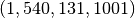$(1,540, 131, 1001)$ using 2 slice sets. Notice also how only geometric coordinates appear in the configuration (the channel dimension is ommited):

"data": {
    ...
    "slicers": [
        {
            "name":               "yz-slices",
            "sizes":              [1, 131, 1001],
            "padded_sizes":       [1, 144, 1008],
            "discard_remainders": false,
            "transpose":          false
        },
        {
            "name":               "xz-slices",
            "sizes":              [540, 1, 1001],
            "padded_sizes":       [560, 1, 1008],
            "discard_remainders": false,
            "transpose":          true
        }
    ]
}

The following options can be set:

name: Slice set name (optional)
sizes: Slice sizes (required). Expects N elements for N-dimensional input data. Setting an element to 1 flattens the slice along that dimension, reducing the dimensionality of the input samples into the network.
padding: Symmetric padding to be added along each dimension (defaults to zero). If $\textrm{sizes=} [h,w,d]$ and $\textrm{padding=}[p_x, p_y, p_z]$ , then slices will have shape $(h + 2 p_x, w + 2 p_y, d + 2 p_z)$ . Cannot be specified together with padded_sizes.
padded_sizes: Total slice size after padding (defaults to sizes). Useful in case the desired padding is asymmetric. Cannot be specified together with padding.
strides: Displacements used when slicing in each direction (defaults to sizes). If smaller than sizes, then slices will overlap.
discard_remainders: Whether to discard regions of the input data which are left over after slicing (default is false, i.e., leftovers are padded up to sizes and added to the sample list).
transpose: Whether to transpose each slice before and after network traversal. Only valid for 2D slices (default is false).

The inference process, including the addition and removal of padding (as well as optional slice transposition), is depicted in the figure below:

HDF5 slice assembly

The predictions obtained by running inferences on the slices can be assembled back into a multi-dimensional array of the same shape as the input, and saved to disk as an HDF5 file. Naturally, this requires that the neural network be geometry-preserving, i.e., the shape of each sample is transfromed as $(C_1,H,W,D) \rightarrow (C_2,H,W,D)$ , where $C_1$ can be different from $C_2$ . Each slice set will result in one dataset in the HDF5 data-structure. To configure HDF5 writing, set the following:

"data": {
    ...
    "hdf5_outfile": "prediction.h5",
    "hdf5_precision": "half"
    ...
}

hdf5_outfile: Name of the output HDF5 file. If set, slice assembly is enabled.
hdf5_precision: Floating-point format used to write the HDF5 datasets. Valid options are “single” for 32-bit floats (default) or “half” for 16-bit floats.

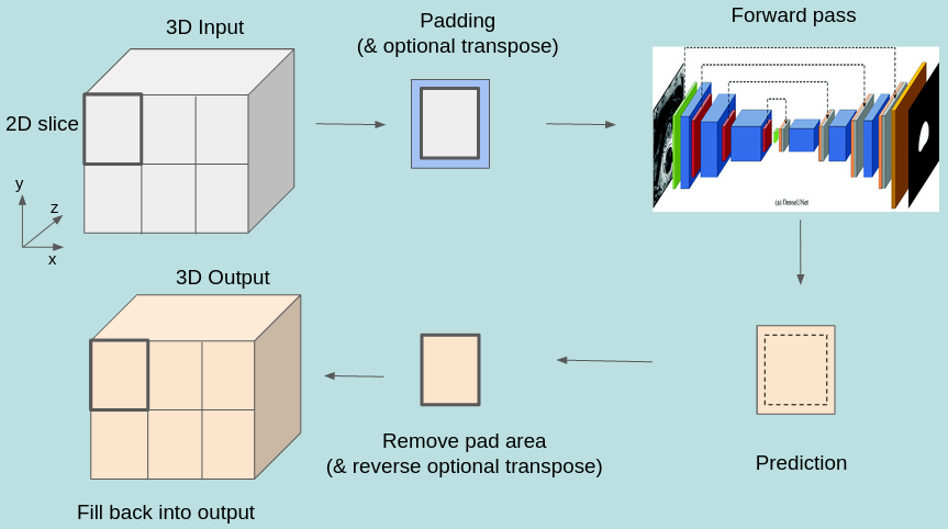
The process of writing data into the HDF5 file is performed in parallel (in case of multi-process execution) and asynchronously, i.e., it happens concurrently with inference in order to maximize throughput. The entire infrastructure for data slicing, inferencing and assembling is depicted in the figure below.

Slicer restrictions:

The input must be one single array (e.g., a single numpy array or a single HDF5 dataset).
The input array must have a channel dimension and its order must be channel-first.
The shape of the output tensor produced by the network can differ from the input shape only in the number of channels, i.e., the neural network must be geometry-preserving.
The transpose option can only be used with 2D slices.

Transforms sub-section¶

The image, numpy and hdf5 data loaders support operations that can be applied to individual 2D samples during training. Notice that:

Operations which are stochastic in nature (e.g., random rotation or random zoom) result in different samples being produced at different epochs, thus providing a mechanism for data augmentation that should enhance training convergence.

Operations which require resizing (e.g., rotation, zooming, resize) apply a linear interpolation scheme by default. If the targets contain discrete data (e.g., masks with integer labels), one should set target_is_mask to true (see Data section), so that a nearest-neighbor interpolation scheme is used for them instead.

The following transformations are supported:

resize: Resizes the sample to a given size using bilinear interpolation.

Usage: resize: [Sx, Sy], where $S_x \times S_y$ is the desired sample size.
center_crop: Crops the sample at the center to a given output size.

Usage: center_crop: [Sx, Sy], where $S_x \times S_y$ is the output size.
jitter_crop: Crops the sample in each direction $i$ by $c \times S_i / 2$ , where $c$ is a random variable uniformly sampled from $c \in [0, C_\textrm{max})$ .

Usage: jitter_crop: Cmax
random_horizontal_flip: Randomly flips the sample horizontally with a given probability $p$ .

Usage: random_horizontal_flip: p
random_vertical_flip: Randomly flips the sample horizontally with a given probability $p$ .

Usage: random_vertical_flip: p
random_zoom: Randomly zooms in by $c \times S_i / 2$ in each direction $i$ , where $c$ is a random variable uniformly sampled from $c \in [0, C_\textrm{max})$ .

Usage: random_zoom: Cmax
rotate: Rotates the sample clockwise by a given fixed angle.

Usage: rotate: phi, where $\phi$ is the rotation angle.
random_rotate: Rotates the sample by a random angle sampled uniformly between $-\alpha$ and $+\alpha$ .

Usage: random_rotate: alpha
convert_color: Converts the image to a different color scheme (given as an openCV color conversion code).

Usage: convert_color: code

normalize: Normalizes the resulting tensor (whose elements are in the $[0,1]$ range) using a given mean $\alpha$ and standard deviation $\sigma$ . That is, for each tensor element $x \in [0,1]$ , it applies: $x' = (x - \alpha) / \sigma$ .

Usage: normalize: {"mean": alpha, "std": sigma}

Below is an example of how to use some of the above transforms. Operations are applied in the same order as they are listed. For that reason, if resize is present, it should usually be the last operation applied, so that all samples going into the neural network have the same size.

"data": {
    ...
    "transforms": [
        { "convert_color": "BGR2RGB" },
        { "random_horizontal_flip": 0.5 },
        { "jitter_crop": 0.1 },
        { "random_rotate": 20 },
        { "resize": [416, 416] },
        { "normalize": { "mean": 0.5, "std": 0.5 } }
    ]
}

The operations listed under transforms will apply to both input and target samples. In order to specify different operations for inputs and targets, the settings input_transforms and target_transforms should be used. For example, if one needs to resize inputs to a different size as the targets, one could do:

"data": {
    ...
    "input_transforms": [
        { "resize": [128, 128] }
    ],
    "target_transforms": [
        { "resize": [16, 16] }
    ]
}

Special-purpose transforms:

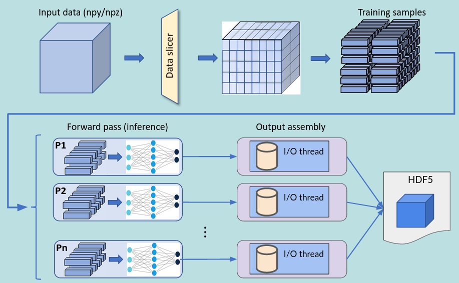
random_patches: Extracts random square patches from the input samples, and makes target samples from those patches. This enables unsupervised training of context encoder networks that learn visual features via inpainting.

This transform can be configured with the number of random patches and their linear size, as for example:

"transforms": [
    { "random_patches": { "number": 100, "size": 10 } }
]

In this case, pairs or input and target samples with 100 patches of size 10x10 are generated during training, like this one:

Checkpoints section¶

In order to save model checkpoints out to disk during training, one must add the checkpoints object to the json config file. This section can also be used to load the model from file before running training. Accepted model file formats are .pt (from libtorch) and .h5 (HDF5 from Keras/TF).

"checkpoints": {
    "save": "./checkpoint_dir/"
    "interval": 10,
    "load": "./model_checkpoint_100.pt"
}

save: The directory to save model checkpoint files into.
interval: When set to $N$ , will save model checkpoints at every $N$ epochs (defaults to 1).
load: A previously created checkpoint file to load the model from.