Applications¶

Image classification¶

In order to train a network for image classification purposes, one must use an image data loader, whose configuration would look something like this:

"data": {
    "input_type": "images",
    "target_type": "labels",
    "input_path": "/path/to/training_data/",
    "test_input_path": "/path/to/evaluation_data/",
    "batch_size": 128,
    "test_batch_size": 200,
    "preload": true,
    "input_grayscale": false,
    "target_grayscale": true,
    "transforms": [
        { "resize": [28, 28] }
    ]
}

The parameters input_grayscale and target_grayscale are specific to the image data loader, and control whether input and target images should be converted to single-channel grayscale (default is false). If the same behavior is desired for both inputs and targets, the single parameter grayscale can be used instead for simplicity.

Specifying target_type: labels triggers the generation of class labels based on directory names. This requires each image file to be inside a directory whose name uniquely identifies that image’s class. (If that is not convenient, one can instead use the parameters training_tag/testing_tag to indicate a directory anywhere in the path underneath which the class name can be found.)

The labels data loader generates targets which are 1D tensors containing a class index (label) in the range $[0, C]$ for each input image in the mini-batch, where $C$ is the number of classes. This requires the loss function to be like the NLL, which expects a target with such shape.

Image segmentation¶

Image segmentation works similarly to classification, except that a target image (mask) must be provided instead of a label for each training example. While the label is a number that is deduced automatically from the input images’ directory names, the target images have to be provided explicitly by means of the target_path and test_target_path parameters of the data loader. These specify the directories where the training and evaluation target images (masks) are located, respectively. Also, since the input and target types are the same in this case (i.e., images), one can simply specify type: images, instead of passing both input_type and target_type. The remaining parameters in the data section are the same as for image classification:

"data": {
    "type": "images",
    "input_path":       "/path/to/training_images/",
    "target_path":      "/path/to/training_masks/",
    "test_input_path":  "/path/to/evaluation_images/",
    "test_target_path": "/path/to/evaluation_masks/"
    ...
}

The target images must be of the same size and depth as the output of the network, and a loss function that expects its input and target to be of the same shape (e.g., MSE, BCE, etc) must be used.

PDE solvers¶

These applications can solve partial differential equations by using the PDE function itself, as well as boundary and initial conditions, as constraints that are enforced by the loss function. It currently supports:

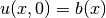
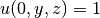
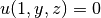
the 1+1D Burgers’ equation (one spatial dimension plus time) with boundary conditions $u(x,0)=b(x)$ and $u(0,t)=0$
the 2D stochastic Poisson equation with boundary conditions $u(0,y)=1$ , $u(1,y)=0$ and $\partial u / \partial \hat n = 0$ on other boundaries
the 3D stochastic Poisson equation with boundary conditions $u(0,y,z)=1$ , $u(1,y,z)=0$ and $\partial u / \partial \hat n = 0$ on other boundaries

Burgers’ PDE solver

The Burgers’ equation in one spatial dimension can be written as

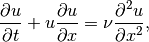
$\frac{\partial u}{\partial t} + u \frac{\partial u}{\partial x} = \nu \frac{\partial^2 u}{\partial x^2},$

where $\nu$ is the diffusion coefficient. When $\nu = 0$ , the Burgers’ equation is said to be inviscid.

The training examples for the network are sets of boundary condition functions $b(x)$ with the form

$b(x) = \frac{1}{2} \left( 1 - \cos(2 \pi c x / d) \right),$

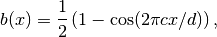
as well as linear superpositions of these raised-cosine functions, where $d$ is the domain size in the x-dimension, and the frequency $c$ is sampled from the interval $[c_{min}, c_{max}]$ using one of the supported distributions (see bc_type parameter below).

The data loader in this case is, therefore, a PDE boundary condition generator, which accepts the following configuration:

"data": {
    "type": "pde",
    "domain_size": 128,
    "num_examples": 64,
    "batch_size": 16,
    "num_test_examples": 8,
    "test_batch_size": 4,
    "bc_frequency": [3, 6],
    "bc_type": "random_uniform"
}

The following parameters can be set:

domain_size (required): The size of the domain in $x$ (the number of time steps is determined by the network).
num_examples: The total number of training examples (i.e., initial conditions). If omitted, the training step is skipped.
batch_size: The number of examples per mini-batch during training (defaults to 64).
num_test_examples: The total number of evaluation examples. If omitted, the evaluation step is skipped.
test_batch_size: The number of examples per mini-batch during evaluation (defaults to 64).
bc_frequency: A range $\mathcal{R} = [c_{min}, c_{max}]$ for the initial condition frequencies $c$ .
bc_type: The method for how to sample the frequencies from $\mathcal{R}$ . Can have the following values:
- random_uniform: Selects $c$ randomly from $\mathcal{R}$ with a uniform probability distribution 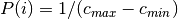$P(i) = 1 / (c_{max} - c_{min})$ .
- fixed_uniform: Selects $c$ sequentially from evenly spaced points in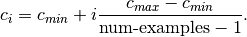 $\mathcal{R}$ , i.e.,
  
  $c_i = c_{min} + i \frac{c_{max} - c_{min}}{\textrm{num-examples} - 1}.$
  
  where $i \in [0, \textrm{num-examples} - 1]$ .

The loss function configuration depends on the specific equation being solved. For Burgers’ PDE, one must set the parameter function as Burgers_PDE, and the following additional parameters are supported:

"loss": {
    "function": "Burgers_PDE",
    "diffusion_coeff": 0.01,
    "boundary_factor": 64
}

diffusion_coeff: The value of $\nu$ (defaults to zero, i.e., inviscid Burgers)
boundary_factor: A multiplier for the boundary + initial condition terms relative to the PDE term. Experiments have shown that a value of 64 works well (defaults to 1).

2D/3D Poisson PDE solver

The Poisson equation is defined as

$-\nabla\cdot (\nu(x,y) \nabla u) = f,$

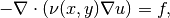
where $\nu(x,y)$ is the diffusivity function. The forcing function $f$ is assumed to be zero. The loss function must be set to Poisson2D_PDE or Poisson3D_PDE:

"loss": {
    "function": "Poisson2D_PDE"
}

To run rmldnn with any of the PDE solver loss functions, add the parameter --app=pde to the command line:

rmldnn --app=pde --config=<json_config_file>

Applications¶

Image classification¶

Image segmentation¶

PDE solvers¶

Table Of Contents

Related Topics

This Page